##Introduction My dissertation, titled The Ahlfors Iteration for Conformal Mapping, lies at the intersection of several areas of pure and applied mathematics, namely complex analysis, conformal mapping, computational geometry and numerical analysis. The main algorithm in the thesis (titled Ahlfors Iteration for the legendary Finnish mathematician Lars Ahlfors) finds a transformation from the circle to any simple polygon. Algorithms have been developed in the past with the same aim, but the novelty in this work lies in the fact that the Ahlfors Iteration is proven to converge, which had not been done for any other method. The mapping found is useful in that it is given by an explicit formula and is conformal, a particularly nice property to have for applications (see below).
The algorithm was implemented in Matlab and made extensive use of the excellent SC Toolbox package written by Tobin Driscoll.
Instead of jumping right into a description of the algorithm, let’s go over some background material needed to gain an understanding of the math behind the iteration.
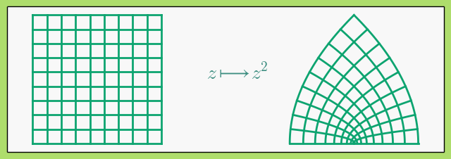
A mapping in the complex plane, \(\mathbb{C}\), is said to be conformal in a region of the plane if at every point in the region it preserves the angles between any lines intersecting at the point. Informally, this means that at small scales a conformal map does not distort shapes. A result of this definition is that conformal maps are continuous and must be one-to-one, i.e. homeomorphisms onto their image. As an example, let’s take the function \(f(z) = z^2\) and see how it transforms the unit square (it is conformal at every point except the origin):
Notice how the 90\(^{\circ}\) angles at the interior intersections of the grid are preserved under \(f\).
In his 1851 PhD thesis, Bernhard Riemann sketched a proof of what would later be called the Riemann Mapping Theorem, which states that for any simply connected open subset \(U\) (think a patch of the plane with no holes and exclude the boundary) of the complex plane, there exists a conformal map from the unit disk to \(U\). This is quite an amazing result when you think about the irregular types of domains you could specify for \(U\), such as one with a fractal boundary.
The downside to Riemann’s theorem is that it is only an existence result. It doesn’t help us find and write down the actual map from the unit disk to our chosen set \(U\). Unless, of course, \(U\) is the interior of a polygon in which case we have the Schwarz-Christoffel Formula.
Edwin Christoffel (1867) and Herman Amandus Schwarz (1869) independently discovered the explicit conformal map from the disk (or, equivalently, the upper half plane) to any simple polygon. We’ll call any such function a SC map. Suppose \(P\) is the interior of a polygon with \(n\) vertices. At vertex \(v_j\) assume \(P\) has interior angle \(\alpha_j\pi\). Then the SC map from the unit disk \(\mathbb{D}\) to \(P\) is given by \begin{equation} S(z) = A\int_0^{z}\prod_{j=1}^n\left(1-\frac{\zeta}{p_j}\right)^{\alpha_j-1}d\zeta + B, \label{eq:SC} \end{equation} where \(A, B \in \mathbb{C}, A\neq 0\), \(p_j\in \partial\mathbb{D}\) and \(S(p_j)=v_j\). The integral can be taken on any path from \(0\) to \(z\). You don’t need to worry about any perceived complexities in the above function. The key points are that we actually can write an explicit formula, this formula is general enough to work for any simple polygon no matter how many vertices there are and, finally, the formula can be efficiently implemented on a computer. Below is an example that illustrates the effect of the disk under one such SC map:
Suppose we fix a polygon and want to find the appropriate version of \eqref{eq:SC}. We know the interior angles, and hence the \(\alpha_j\). The constants \(A\) and \(B\) control the scaling and location of the polygon, and therefore can be easily solved for last once we have the correct shape of the polygon. This leaves us with the unknown \(p_j\). The issue of finding these parameters, dubbed the Schwarz-Christoffel parameter problem, is exactly what the Ahlfors Iteration solves.
In order to arrive at the solution to the SC parameter problem we will make iteratively better and better approximations to the true solution. But what do we mean by better? If we have a guess for the parameters, then the image polygon we get will have the correct interior angles but the side lengths (more precisely, the side length ratios) will be off. In order to measure how far off we are we need to introduce a new class of functions: Quasiconformal Maps.
###Quasiconformal Maps Since we defined conformal maps as functions that don’t deform shapes at small scales you may have guessed that quasiconformal maps, or QC maps for short, introduce some distortion. If so, you’ve guessed right. More formally, a map \(f\) between domains in \(\mathbb{C}\) is quasiconformal if it satisfies the Beltrami equation \begin{equation} \frac{\partial f}{\partial\bar{z}} = \mu(z)\frac{\partial f}{\partial z}, \label{eq:beltrami} \end{equation} where \(\mu\), called the (complex) dilatation, is a complex function whose absolute value is less than 1. Once again, you don’t need to concern yourself with the details of \eqref{eq:beltrami}, just know that when \(\mu\equiv 0\), \(f\) is conformal, and the higher the value of \(|\mu(z)|\) the more distortion \(f\) introduces at \(z\).
A simple example of a QC map, and the only one we’ll need for the algorithm, is the complex affine function \begin{equation} L(z)=az+b\bar{z}+c, \label{eq:affine} \end{equation} where \(\bar{z}\) is the complex conjugate of \(z\). Using \eqref{eq:beltrami} it is easy to see that the dilatation, \(\mu_L\), of \(L\) is constant and equal to \(\frac ba\). Geometrically, \(L\) causes a shearing effect on the plane and the higher the dilatation the more pronounced the shearing. Below illustrates how various forms of \(L\) map the solid triangle to the dashed one and the corresponding complex dilatation. Notice that as the solid triangle becomes more similar to the dashed the more the dilatation decreases.
We claimed before that QC maps would give us an idea of how close an approximate guess to the parameter problem is to the true solution. In order to see that this is the case, suppose we have a guess for the parameters and the corresponding SC map, \(S\), to an approximate polygon \(P’\). Let \(P\) be the true polygon we’re trying to find the map for. If we can construct a QC map \(F\) from \(P’\) to \(P\) with dilatation \(\mu_F\), then the composition \(S\circ F:\mathbb{D}\rightarrow P\) is still quasiconformal with dilatation \(\mu_F\). Since the complex dilatation measures how close a map is to being conformal, we see that if \(\mu_f\equiv 0\) then our guess for the parameters is actually the true solution. So if we can iteratively decrease the magnitude of the complex dilatation towards 0, we can get closer and closer to the true solution.
But how do we find a QC map from our approximate polygon to the true polygon? We already noted that QC affine maps can be constructed to map triangles to triangles. So in order to map polygons we just decompose them into triangulations and paste together the affine maps to get a piecewise QC affine map.
###Triangulations A triangulation of a polygon is simply a decomposition into non-overlapping triangles whose vertices are also vertices of the polygon. A particular triangulation does not have to be unique. However, there is a particular type of triangulation that provides a decomposition with triangles whose angles are not too acute, which is convenient not only for the proof of convergence of the Ahlfors Iteration but also for the numerical implementation. This type of triangulation is called a Delaunay triangulation. A triangulation is said to be Delaunay if the circumcircle of each triangle (the unique circle passing through each of the triangle vertices) contains no other vertex of the polygon. Here are two Delaunay examples:
Now that we know about triangulations we can construct the aforementioned QC map from an approximate polygon to the true polygon. We assume that both polygons can be triangulated coherently, i.e. each triangle in the approximate polygon and its vertices matches up with a triangle in the target polygon triangulation and its vertices. Then for each triangle in the approximate polygon we construct a complex affine map \eqref{eq:affine}. Pasting these maps together gives a QC map \(F\) from the approximate polygon to the target polygon. The maximum dilatation is the highest \(|\mu_L|\) amongst the affine maps of the triangles.
##The Ahlfors Iteration Let’s turn now to the proven solution of the Schwarz-Christoffel parameter problem, the Ahlfors Iteration. The iteration is in the same vein as Newton’s Method in that it is based on a first-order function expansion and the convergence to the solution is quadratic (in our case the convergence is in QC space, i.e. if we have a guess for the parameters and the QC affine map constructed above has dilatation at most \(\epsilon\) then the next guess will have error \(O(\epsilon^2)\)). For further details and proofs check out the source.
###Algorithm To start, we need to move our parameters from the unit circle to the real number line in the complex plane. There’s no difficulty doing this since we can use the inverse Cayley transform, which is conformal and maps \(\mathbb{D}\) to the upper half plane, \(\mathbb{H}\). This step is necessary to apply the update step in the iteration. The parameters will be moved on the real line and then mapped back to the disk and we can use the SC map above to get the updated approximate polygon.
For the sake of brevity, I’ve changed the iteration presented here slightly from how it is written in my thesis, where instead of moving a fixed set of parameters each parameter is renormalized using cross-ratios in order to avoid the “crowding effect” of parameters that causes numerical problems. See this article by Driscoll and Vavasis for an overview of the crowding problem and how to get around it using cross-ratios.
Suppose \(P\) is a simple polygon with \(n\) vertices for which we would like to solve the SC parameter problem. The Ahlfors Iteration is as follows:
Before proceeding to some examples you may be curious as to exactly how the integral in \eqref{eq:update} can be calculated in a reasonably fast way since the integral is taken over the entire complex plane. However, there are some simplifications and numerical techniques we can use to greatly simplify the task at hand.
Because we extended the function \(f_k\) to the whole plane we can do the reverse and simplify the domain to \(\mathbb{H}\). Then since we know the exact form of \(S_k\) we can make a change of variables and integrate instead over the polygon \(P_k\).
We then use Green’s theorem (no relation) to integrate not over the two dimensional polygon but the one dimensional boundary of the triangulation. Now we have a collection of one dimensional integrals that can be numerically approximated using Gaussian quadrature, which is a much better situation to be in than having to integrate over the entire plane.
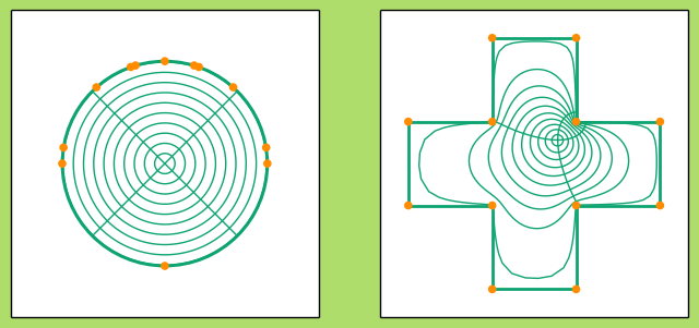
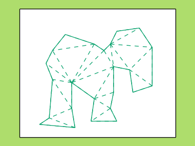
###Examples Below are a few examples of the Ahlfors Iteration in action. The top left image shows the movement of the prevertices at each iteration. The top right shows the approximate polygons in solid green approach the dashed line target polygon. You may notice that three vertices never move. There’s nothing tricky going on here, it is just a fact from the conformal theory that you can always send any three points to any three points conformally. So in reality if we have a polygon with (n) vertices we only need to solve for (n-3) prevertices.
Finally, the bottom image plots the maximum dilatation of the piecewise affine maps on the triangulations. Recall that these numbers measure the accuracy of the iteration and the lower the value the closer we are to the true parameters.
##Applications The Schwarz-Christoffel mapping has many useful applications in applied mathematics. These areas include electrical engineering, fluid mechanics, and mesh generation. The most basic problem usually breaks down to solving Laplace’s equation on a complex polygonal domain where the problem simplifies when an SC map is employed. For a detailed description of some applications and many references to more see Schwarz-Christoffel Mapping by Driscoll and Trefethen.